
Balancing Level Difficulty in Hybrid-Casual Puzzles using ML and System Modeling
How can we predict the win rate of a level using machine learning on a dataset prepared with simulated player behavior?


It’s been a few months since I last published a new article. But here we are! This topic has been on my mind for a long time, and I finally had time to share some important concepts with you. I believe you’ll find it useful!
Hybrid-casual puzzles are rising stars, and the trend seems to continue increasing steadily. In this blog post, we’ll explore a slot-limited puzzle game to model a system that controls level difficulty, and finally, we’ll create a machine learning model to predict the win rate of levels based on a given configuration.
Before we move on, here is Stick Jam, a prototype I prepared for this article:
I inspired by Voodoo’s Slinky Jam to prototype Stick Jam. You can watch the video below to get an idea of its gameplay:
We will discuss 5 major topics throughout the article:
Game elements and rules, discussed in Introduction section.
Theoretical background of system design in Stick Jam, discussed in Understanding Variable Relationships section.
Controlling level difficulty, discussed in Difficulty Adjustment Algorithm section.
Modeling player behavior and simulation setup, discussed in Simulation Design section.
Win rate prediction for levels, discussed in Predicting Outputs with Machine Learning section.
Introduction
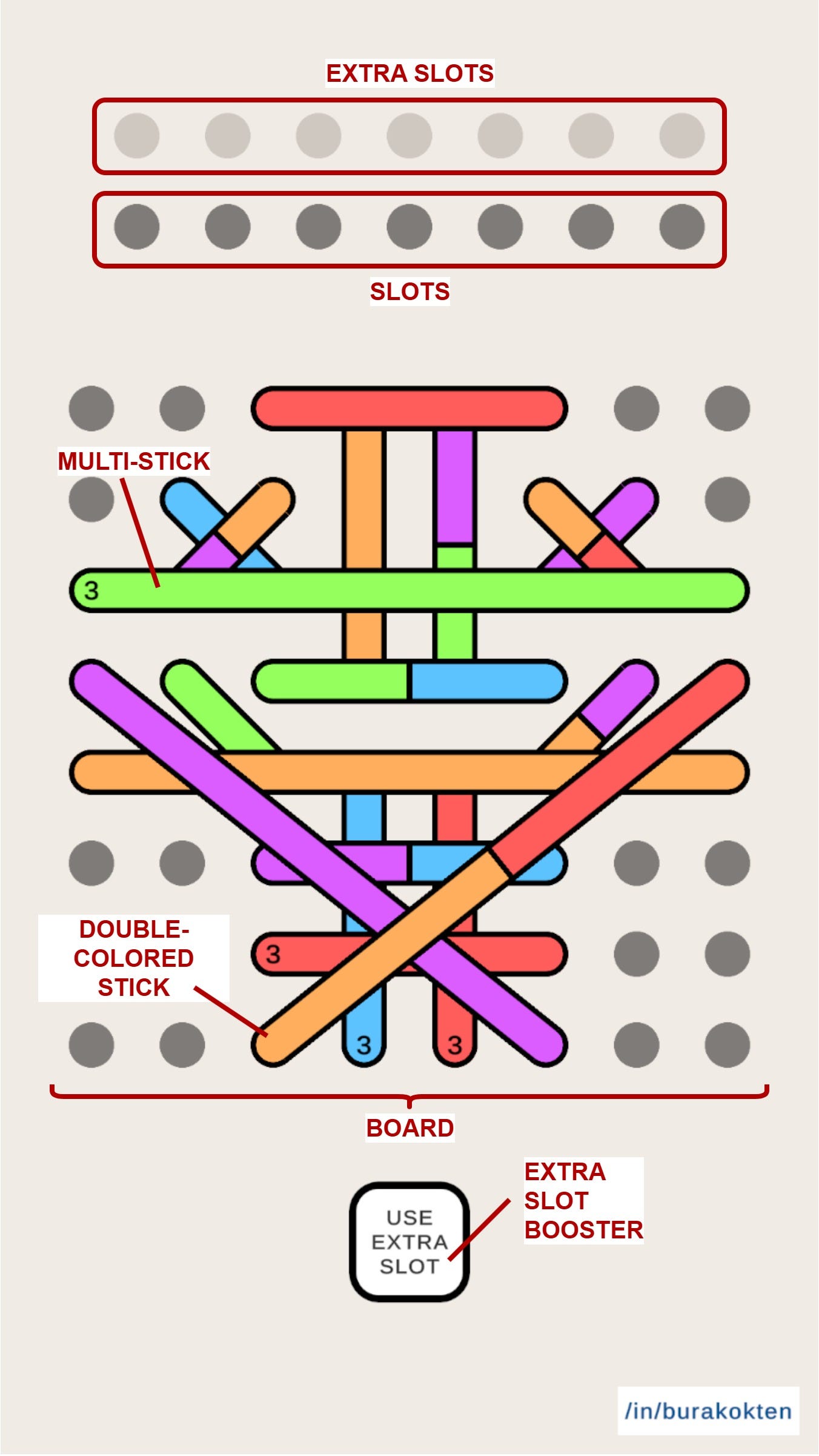
Stick Jam consists of 2 main parts that players interact with:
There is an NxM board with sticks on it. The minimum board size is 3x3 and the maximum is 8x8, although there is no theoretical upper limit.
There are 2x7 slots. The bottom row is for placing stick colors collected from the board, and the top row is for extra slots. When the “Extra Slot” booster is used, the rightmost color in the bottom row moves to the top row. I also decided to limit the number of extra slots, even though it’s not strictly necessary.
Players try to collect all sticks by checking for color matches on the slots. When 3 of the same color are placed in the bottom slots, they form a match and are removed. If the bottom slots become completely full without any match, the level fails. If players collect all sticks without letting the bottom row fill up, the level is completed.
Levels are generated dynamically based on a difficulty configuration, which we will discuss in the next sections. Therefore, no players encounter the same color sequence.
Special Sticks
Double-colored stick: It represents 2 sticks at once, so when collected, it occupies 2 slots.
Multi-stick: It has a counter that shows how many sticks must be collected before it is completely removed from the board.
Double-colored sticks tend to make the level finish faster, but also increase the failure probability. They require careful placement, otherwise, it’s easy to end up in a state where only one slot is available but all collectible sticks are double-colored.
Multi-sticks, on the other hand, introduce a bit of chance by hiding the next color, which can make players feel either lucky or frustrated.
Understanding Variable Relationships
Designing a system starts with understanding the internal role of each variable added to it. Then it continues with identifying relationships between variables, observing how they affect system behavior, what hidden features they reveal, and how they respond when a new variable is introduced. These relationships may stem from mathematical dependencies as well as algorithmic constraints. In our case, we’ll see that both aspects must be considered, and each contributes to data-driven level design.
Level difficulty directly depends on how we control the frequency of color-matching in the slots. If the system arranges colors in a way that requires more than the available slots, we call it a “hard level”, otherwise, it's an “easy level”. The transition between difficulty levels is gradual and controllable. This transition is also the key to dynamic difficulty adjustment.
Before diving into the algorithm, let’s start by exploring each variable and their theoretical relationships to define the system’s limitations:
where N_s is the number of slots and N_c is the number of unique colors. This inequality guarantees a solution for the worst-case scenario, which is when there is only one stick to choose from each time after players remove a stick from the board.
If the number of slots is 7, then a solution is guaranteed for up to 3 unique colors in the worst case.
where N_st is the target number of slots used in the color path generation algorithm. This inequality basically states that a solution is always guaranteed when the condition is met. We will discuss how it works when we model the algorithm in the next section.
where N_stick is the number of sticks in a level. It must be a multiple of 3, and the number of unique colors cannot exceed the dividing the number of sticks by 3.
where N_stick,a,avg is the average number of available (ready to collect) sticks from the beginning to the end of the level after each stick is collected. M is the number of moves needed to solve the level. It is equal to N_stick.
Increasing the average number of available sticks gives players more options to choose from and makes the level easier.
Difficulty Adjustment Algorithm
1. Introduction
We discussed game elements and variable relationships up to this point. I strongly recommend reading the previous section before diving into this one. Now, it’s time to bring everything together to create a difficulty algorithm controllable by a few parameters.
First, we should define which variables we can directly change, what output we should expect, and how we can measure it. Measurement is very important, otherwise system design cannot reach its full potential. Even worse, it may turn into a useless model that wastes your precious time.
When we look from the player’s perspective, if any visible layer of sticks shares the same colors, it means it’s easier to select sticks for color-matching. If these sticks don’t share many colors, it forces players to think strategically before removing a stick from the board. Thus, the controlled output should be the stick colors based on the layer they are standing on.
An important point I want to highlight is that we should expect different outputs for different inputs within the same level. This means that stick placement or distribution in a level doesn’t directly affect the output. In the next sections, we’ll see that it affects how we perceive difficulty across levels.
Now, the question is which variables can control the output? If it were possible to change the number of slots dynamically for each level, it could be useful. However, this also has high potential to be very annoying for players. Instead, we can control its counterpart. By adjusting the target number of slots instead of the actual number, we can take advantage of slot-dependent control without modifying the real slot count. When the target slot count is less than the actual slots, the level tends to be easier. If it's greater, the level becomes harder and sometimes it becomes even impossible to solve. I’ll show how this works in this section, so keep reading!
The other variable we can directly control is the number of unique colors. Levels with too few colors would be very boring and lack visual variety. However, randomly distributing colors could naturally lead to quick failure. We will use unique colors and target slots in a way that allows more colors for easier levels and fewer colors for harder ones. This is the level of flexibility we aim to achieve.
You will observe how variables can change the difficulty of the same level in the following videos:
This level is generated with 8 unique colors and only 4 target slots. It can be considered an easy level.
Again, 8 unique colors. But this time, the target slots are 8. Can you tell the difference?
Finally, 8 unique colors and the target slots are increased to 12. It’s basically a paywall level!
The beauty of this algorithm is that it still preserves randomness, so refreshing a level produces completely different color sequences while keeping the average difficulty the same.
It can also be applied to the special sticks defined earlier. Here is an example of a multi-stick level:
This level has 7 unique colors with 7 target slots. Look how the upcoming colors help ease the slots!
2. How It Works
There are 3 major algorithms working together:
Sorting sticks based on their parent counts.
Creating a color path based on the number of unique colors and the number of target slots.
Assigning colors to sticks.
Sorting sticks is the easiest part. When a level is designed, the only requirement is to check which sticks are parents of which. A stick may have more than one parent, or it may have none. If it doesn’t have a parent, it means the stick is ready to be collected.
Color path generation is a bit tricky. Take a look at the following flowchart:
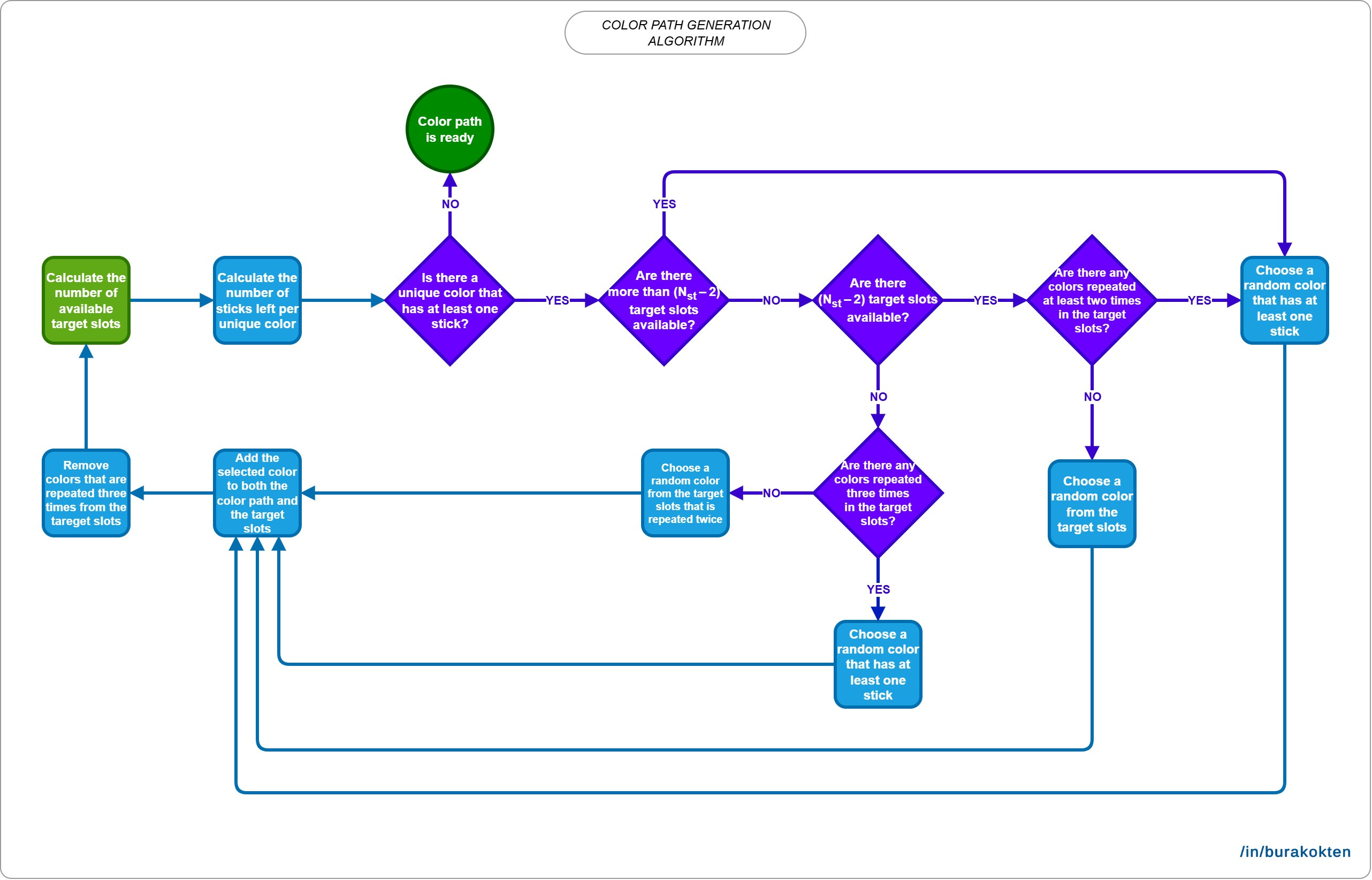
The goal of this algorithm is to create color matches before the theoretical slots are completely filled. It guarantees at least one way to remove sticks from the board, as expected. We’ll look at how it’s affected by the average number of collectible sticks in the next sections. You can also check the Understanding Variable Relationships section for a discussion of the theoretical background.
Here are some examples of generated color paths with different configurations. Each number represents a unique color id:
Generated color path for 7 target slots and 10 unique colors:
7, 0, 5, 2, 9, 5, 5, 3, 9, 9, 6, 6, 6, 1, 7, 7, 8, 8, 8, 4, 0, 0, 1, 3, 1, 2, 4, 4, 3, 2, 8, 2, 6, 4, 0, 4, 4, 3, 2, 2, 9, 0, 0, 5, 8, 8, 7, 6, 6, 1, 1, 1, 7, 9, 9, 3, 5, 7, 3, 5
Generated color path for 12 target slots and 10 unique colors:
6, 5, 2, 9, 4, 0, 3, 1, 7, 8, 9, 9, 1, 2, 2, 8, 5, 1, 3, 4, 5, 7, 6, 3, 0, 4, 0, 8, 6, 7, 3, 2, 6, 4, 7, 5, 1, 8, 9, 0, 5, 5, 1, 6, 6, 9, 3, 1, 2, 7, 9, 0, 8, 3, 4, 7, 0, 2, 8, 4
As seen in the generated paths, the algorithm tries to keep the number of slots at the target count and creates color matches just before it becomes completely full.
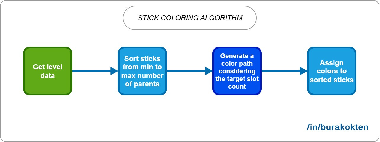
Finally, we should assign the generated colors to sticks by considering the number of parents in ascending order. After this step, the level is ready to play!
These algorithms can also be applied to dynamically control level difficulty. Assume that players continue to fail a level. It’s now possible to decrease the difficulty automatically after N attempts, based on your data and what you consider the sweet spot.
Although I didn’t introduce a flexibility variable, it’s also possible to control randomness with such an addition. However, that would be too much for this article, and it’s always better to model your system step by step. After each step, observe the real-world behavior and then calibrate the parameters.
Simulation Design
Without testing the algorithm in real-world, it’s not really possible to predict the results accurately. Unlike what we expect theoretically, systems may behave differently when deployed in a real environment. On the other hand, testing with real players is often costly, especially in terms of time. An alternative approach is to simulate the real environment with a proper setup. Although it’s not a 100% replacement for real-world testing, it provides valuable insights into how solid your system is and can serve as a reference point for adjusting configurations before real tests.
I decided to use simulations to generate a batch of data, as shown in the table below. Here is the configuration used:
Number of levels: 17 (with various number of sticks)
Target slots: 4 to 12
Unique colors: 3 to 12
Simulated players per level: 1000
Collected data:
Average number of collectible sticks
Win rate
Total 1449 rows
Note that when the number of sticks cannot support enough unique colors for the given configurations, as discussed in the Understanding Variable Relationships section, those setups are skipped.
None of the simulated players are allowed to try a level more than once. Thus, I didn’t focus on the number of attempts, but rather on the win rate. However, it’s possible to calculate the average attempts per virtual player by dividing one by the win rate.
The table below shows 10 rows of randomly selected data from the dataset:
Modelling Player Behavior
Designing a solution checker algorithm is a good approach if you want to ensure that a level has a solution. However, it lacks two important things. First, it doesn’t tell us how players perceive the level's difficulty. Second, it’s not applicable when we intentionally introduce unsolvable levels (e.g. when we expect players to use boosters earned through gameplay). So, what should we do? The best approach is to model player behavior by thinking like a player. Put yourself in the player’s position and try to understand: How would you play? How would you try to solve the level without using boosters? And finally, what limitations would you have as a player? A solver algorithm can try multiple paths to find a solution or the best one, but a player doesn’t have that luxury.
In our case, let’s look at how a player might play and what limitations they face:
They must follow the gameplay rules. There are no exceptions.
They can decide which sticks to remove from the board based on visible sticks. They cannot predict the color of hidden or upcoming multi-sticks.
They can also decide which sticks to remove based on the state of the slots. They may consider whether there is a color match, whether a slot is almost full, or whether it is empty.
They can combine these observations to choose the best stick to remove.
Even if they construct a strategy, they cannot keep all game states in mind, unlike a solver that traces every possible path. Instead, they have limited ability to track possible moves, and this is the core of the player model.
Consider the following flowchart of the player model:
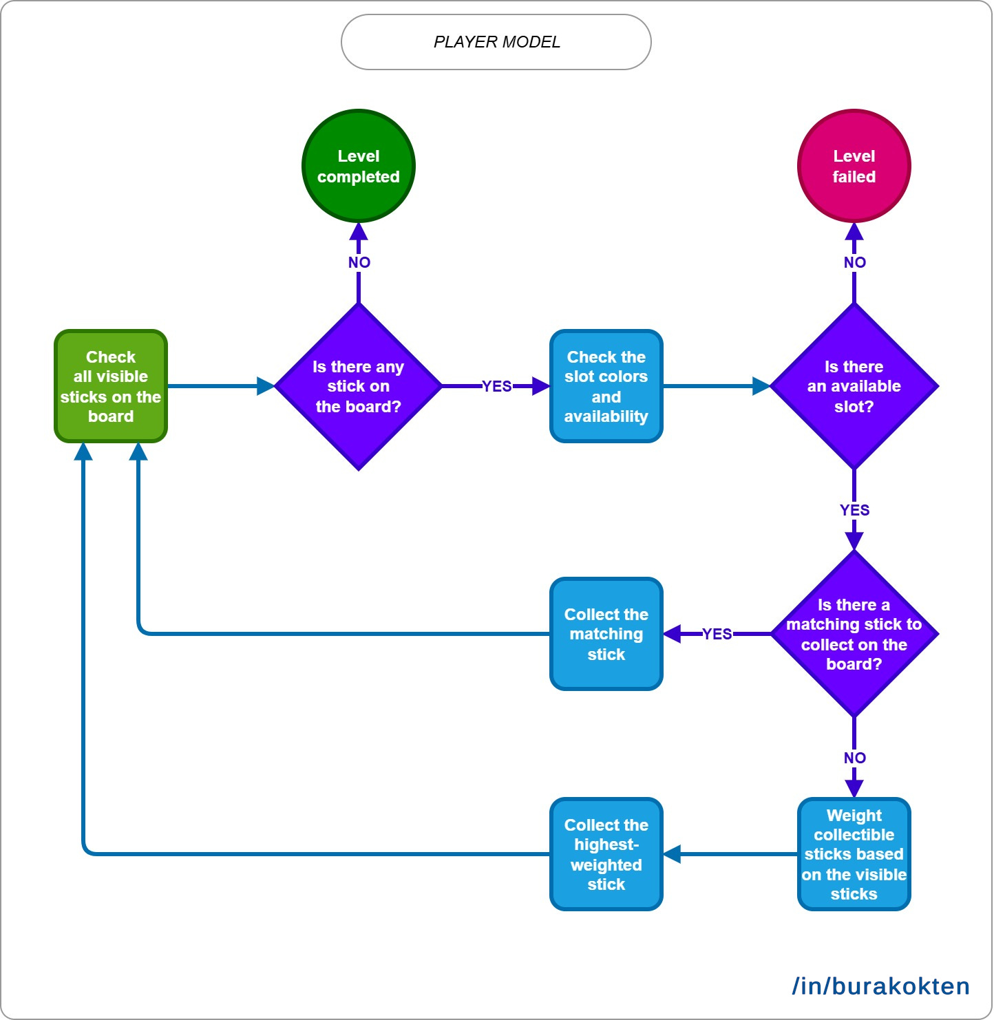
As a reference, I designed and played many levels, observed how I reacted while collecting sticks, and took notes. Since it’s not the main focus of the article, I won’t go into every detail of how it works. However, as shown in the flowchart, it uses a type of weight-based algorithm to decide which stick to collect. This allows the algorithm to behave more like a real player rather than a solver.
Predicting Outputs with Machine Learning
As we discussed earlier, the whole point of the simulation was to create a dataset for the machine learning model. Our goal in this section is to find a model that fits the dataset and makes sufficiently accurate predictions for win rate. This will then help us predict the win rate before we even begin designing a level.
It is indisputable that if we had real player data, it wouldn’t result in a dataset this clean. What we would normally expect is noisy data with various disturbances, such as failures caused by bugs, incorrect or missing analytic events, targeting the wrong audience, and so on. However, since we are using simulation results, we assume the dataset contains no noise other than the natural variation in simulation outcomes. I tried to minimize this by increasing the number of simulated players to 1000, but it cannot be completely eliminated.
As the ML model, I chose Gradient Boosting for win rate prediction. The selected features were N_st, N_c, N_stick,a,avg, and N_stick. During cross-validation on the training data, the average R² score was 0.938 with a standard deviation of 0.011, and the RMSE was 0.098. On the test set, these values were 0.952 for R² and 0.086 for RMSE. I also tested different hyperparameter configurations to avoid overfitting as much as possible. The model appears to explain 93.8% of the variance in win rate with the given feature set, and its performance was even better on the test data. The higher R² score on the test set is noteworthy, as this may be due to the simplicity of the data structure or the effect of chance. When tested with real-world data, this outcome may very well reverse. Feature contributions were 46.8%, 21.1%, 19.5%, and 12.6% for N_c, N_st, N_stick,a,avg, and N_stick, respectively. Keep in mind that while the results are promising for this article, larger datasets and further tuning are needed in real-world scenarios for better predictions.
Let’s continue with the predictions. Since it’s not possible to include every combination here, I decided to choose a few configurations that make sense to examine.
Configuration 1:
N_s = 7
N_stick,a,avg = 4
N_stick = 42
Result:
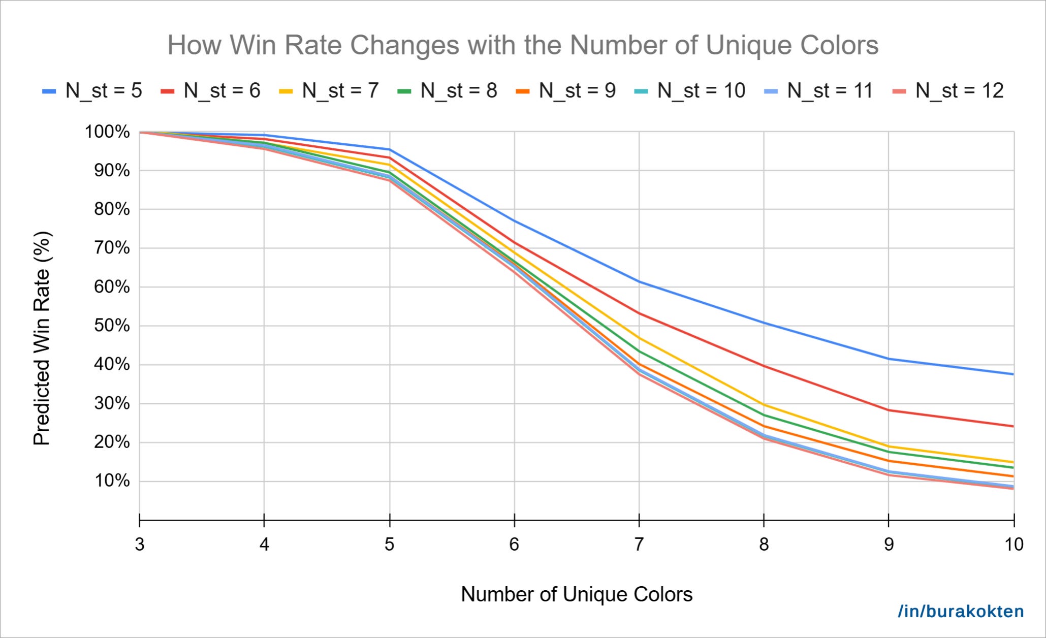
In the chart above, N_stick,a,avg, N_stick, and N_s are held constant, while N_c and N_st vary. As expected, when the number of unique colors is 3, the outcome becomes completely independent of the target slots. This theoretically ensures a 100% win rate, as discussed in the Understanding Variable Relationships section.
As the number of unique colors increases, the win rate decreases. However, maintaining a higher number of target slots slows down this decline. For example, when the number of unique colors is 10, the win rate with 5 target slots is nearly four times of the lowest value.
It’s also interesting to observe that continuously increasing the number of target slots eventually stops making a difference. This is expected, because when the target slot count is lower than the actual number of slots, the solution becomes more obvious (and the level easier). But as we keep increasing the target slot count, the added difficulty loses meaning, as players tend to fail faster.
Another notable point is that the win rate is predicted to be very high for all target slot values until the number of unique colors reaches 6. I assume the average number of collectible sticks helps balance the negative impact of increment in the target slots. However, this would need further testing with new levels to confirm.
Configuration 2:
N_st = 7
N_s = 7
N_stick = 42
Result:
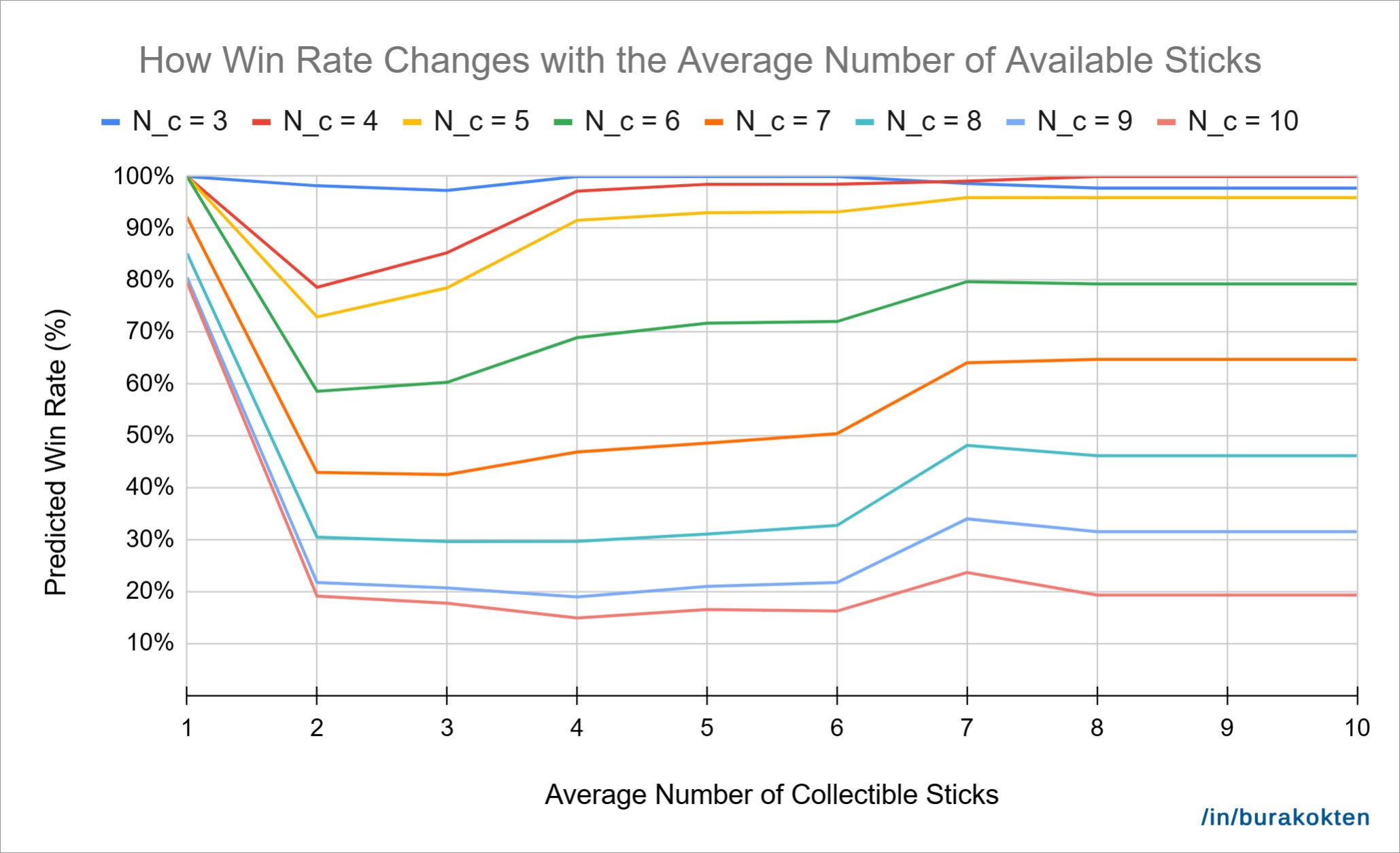
In this second chart, we observe how the average number of collectible sticks affects the win rate for different numbers of unique colors. N_st, N_s, and N_stick are held constant. The first observation is that increasing the number of collectible sticks initially causes a sharp drop in the win rate.
The reason is that when the average number of collectible sticks is 1, there is only one possible move at a time. This removes the influence of player decision-making. However, when there are two or more options, the number of unique colors starts to heavily impact the outcome.
As we continue to increase the average number of collectible sticks, we also see a rise in win rate. This aligns with the theoretical expectation that getting closer to 2*N_c+1 improves win probability. This effect is especially noticeable when the number of unique colors is low.
On the other hand, the model seems unable to accurately capture win rate when the average is 1, as the theoretical expectation is 100% in that case.
As we observed, level design cannot be considered independent from system design. Relying solely on randomness turns the game into a black box. That’s why measurement is like a two-sided coin: one side is modeling level configurations and building a controllable difficulty system, and the other is collecting analytical data. Combining both allows you to make better predictions and more importantly, understand which variables affect player engagement. I would also recommend reading my other blog post Designing Tripeaks Solitaire Levels with Predictable Outcomes which covers a similar topic.
This was my third article, and I really enjoyed preparing it. I hope you liked it too.
See you next time!